DeDaL
Data-driven network layout
Skills
- Java
- Networks
- PCA
- Data viz
Project of DeDaL was born in 2014 (or long before) in a context of cancer research in the lab of Computational Systems Biology of Cancer in Institut Curie in Paris in the mind of my research advisor Andrei Zinovyev.
The idea was to develop a tool that would combine multidimensional meta data associated with network and network itself in a form of an intelligent layout. We achieved it through performing PCA and Elastic Map (non-linear version of PCA) on the meta dataset and mapping network connexions into this MDS layout.
The difference between DeDaL and other MDS layouts available, it that DeDaL uses meta data and not the network structure in order to perform the layout. It also contains additional and more advanced features like network smoothing, alignment and morphing. DeDaL helps to interpret and visualize multidimensional data associated with network.
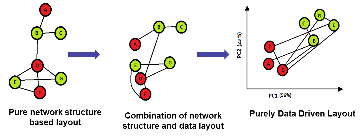
Cartoon representing idea of DeDaL
Today, DeDaL is a piece of software, I developed in Java together with A. Zinovyev, that can be used in Cytoscape 3.0 network visualization interface. It has been applied to a number of biological data which resulted in publication in BMC Systems Biology. Together with DeDaL website that contains full description and step-by-step tutorial and github repository, the software is well documented and open.
However, DeDaL finds its application not only in biological data. Here I post a little demo of DeDaL applied to International Currencies 1890-1910 data from Flandreau, M. and C. Jobst to encourage you to try it out with different data.
International currencies dataset
‘For better or worse – and opinions differ on this – the choice of which language and which currency is made not on merit, or moral worth, but on size.’ (Kindleberger, 1967, p. 11)
The dataset gives measures for the international role of 45 currencies between 1890 and 1910 as well as a set of variables that can explain the relative position of these currencies. Data have been collected for the years 1890, 1900 and 1910. The exchange structure matrix is complete from an empirical point of view, including virtually all currencies of the world in 1890-1910. It also has the nice conceptual feature to identify two different exchange markets for a given currency pair, corresponding to the home countries of the two currencies involved.
The information on foreign exchange refers to ordered country pairs, i.e. for every country pair there are two observations: (1) whether the foreign exchange markets in the first country trade the second country’s currency and (2) whether the foreign exchange markets in the second country trade the first country’s currency. The data file is structured accordingly. The first two columns country_A and country_B identify the country pair, where country_A gives the location of the foreign exchange market and country_B the home country of the currency traded. There is information on 45 countries/currencies, yielding a total of 45*44 = 1980 country pairs.
Article by Flandreau, M. and C. Jobst describes the world currency market based on the set of variables:
- dist: log distance as the crow flies between the cities with foreign exchange markets in country_A and country_B.
- bitrade gives total trade between country_A and country_B in thousand US dollars.
- gold is an indicator variable =1 if country_A has a currency convertible in gold in 1900 and 0 otherwise.
- debtburden is the ratio of government debt over government revenues in 1900.
- rlong is the secondary market yield for gold denominated government debt in 1900.
- rshort1900 is the market rate for 3 month lending, in most cases the discount rate for 3 month commercial paper in 1900.
- rshort1890 same as above for 1890.
- rgdp and rgdpcap give the log 1900 real gdp and the log real gdp per capita.
- poldemo reproduces the index of democracy (ID) of the Polyarchy dataset developed by Vanhanen (2000) for 1900.
- coverage is the logarithm of the number of currencies traded in country_A.
Detailed information can be found in the intro document.
Hands on
Here, using DeDaL I will try to see how much we can learn about currency market without previous knowledge in economy, based on the network and metadata associated with each country.
Firstly, I will import the raw data from the website. I am skipping first 9 lines that contain the intro text:
The international circulation of currencies 1890-1910 Please cite as: - When using the network data for 1890, 1900 or 1910: Flandreau, M. and C. Jobst (2005), ‘The ties that divide: a network analysis of the international monetary system 1890–1910’, Journal of Economic History, vol. 65(4). - When using the explanatory variables for 1900: Flandreau, M. and C. Jobst (2009), ‘The empirics of international currencies: Networks, history and persistence’, The Economic Journal, vol. 119(April).
And we can have a look at the imported table with function head printing first 5 lines.
file <- "http://eh.net/wp-content/uploads/2014/08/flandreau_jobst_internationalcurrencies_data.txt"
raw_data <- read.delim(file, header=T, skip=9)
head(raw_data)
## country_A country_B quote1890 quote1900 quote1910 colony dist
## 1 ARG AUH 0 0 0 0 9.374816
## 2 ARG AUS 0 0 0 0 9.360207
## 3 ARG BEL 1 1 1 0 9.330780
## 4 ARG BRA 0 1 1 0 7.613854
## 5 ARG CAN 0 0 0 0 9.105001
## 6 ARG CEY 0 0 0 0 9.600443
## bitrade gold debtburden rlong rshort1900 rshort1890 rgdp rgdpcap
## 1 5909.76 1 6.844985 7.01 7.06 9.33 16.37536 7.92154
## 2 1258.74 1 6.844985 7.01 7.06 9.33 16.37536 7.92154
## 3 127361.20 1 6.844985 7.01 7.06 9.33 16.37536 7.92154
## 4 65335.41 1 6.844985 7.01 7.06 9.33 16.37536 7.92154
## 5 5073.84 1 6.844985 7.01 7.06 9.33 16.37536 7.92154
## 6 0.00 1 6.844985 7.01 7.06 9.33 16.37536 7.92154
## poldemo coverage gold_B debtburden_B rlong_B rshort1900_B rshort1890_B
## 1 0.3 1.94591 1 5.222065 4.01 4.58 4.48
## 2 0.3 1.94591 1 6.065920 3.12 5.50 7.00
## 3 0.3 1.94591 1 4.882136 3.15 4.09 3.18
## 4 0.3 1.94591 0 5.516892 6.97 9.20 6.30
## 5 0.3 1.94591 1 6.784091 3.61 6.50 6.50
## 6 0.3 1.94591 1 1.362319 3.25 NA NA
## rgdp_B rgdpcap_B poldemo_B
## 1 18.14368 7.39388 0.87
## 2 16.52440 8.29729 6.37
## 3 17.02921 8.22443 10.66
## 4 16.31639 6.51915 0.22
## 5 16.58091 7.97625 8.58
## 6 15.43420 7.16240 0.00
In order to import the network into DeDaL we will need 2 files:
- with node to node connexions to construct the network (
country_Atocountry_B) with edge attributes - table with meta data containing information about nodes (
country_A var1 var2etc.)
I will try initially to take a look at all the connexions that occurred, taking into account the link if trading was active in any year (observed), especially because we do not have detailed data for all time points, then I get rid of time information (3,4,5). I use package dplyr:
suppressMessages(library(dplyr))network_table<-raw_data%>%filter(quote1890==1 | quote1900==1 | quote1910==1)%>%select(country_A:bitrade,-(quote1890:quote1910))
network_table$colony=as.factor(network_table$colony)
summary(network_table)## country_A country_B colony dist bitrade
## DEU : 14 GBR : 44 0:261 Min. :5.373 Min. : 0
## NLD : 13 FRA : 38 1: 12 1st Qu.:6.783 1st Qu.: 30550
## DNK : 12 DEU : 31 Median :7.482 Median : 93208
## USA : 12 USA : 19 Mean :7.674 Mean : 248059
## FRA : 11 BEL : 16 3rd Qu.:8.881 3rd Qu.: 286344
## GBR : 10 NLD : 16 Max. :9.855 Max. :3545484
## (Other):201 (Other):109This table is ready to export.
write.table(network_table, "network_table.txt", row.names=FALSE, col.names = TRUE, quote=FALSE, sep="\t")Then I create table with information about each country. I select a unique entry by country as in Cytoscape we don’t need distinction between country A and B.
countries_data<-raw_data%>%select(country_A:coverage,-(country_B:bitrade))%>%distinct(country_A)%>%rename(country=country_A)
countries_data$gold=as.factor(countries_data$gold)
dim(countries_data)
## [1] 45 10summary(countries_data)## country gold debtburden rlong rshort1900
## ARG : 1 0:19 Min. : 0.000 Min. : 2.550 Min. : 3.210
## AUH : 1 1:26 1st Qu.: 1.759 1st Qu.: 3.290 1st Qu.: 4.835
## AUS : 1 Median : 4.611 Median : 3.810 Median : 5.870
## BEL : 1 Mean : 4.943 Mean : 4.962 Mean : 6.073
## BRA : 1 3rd Qu.: 7.257 3rd Qu.: 6.100 3rd Qu.: 6.750
## CAN : 1 Max. :14.656 Max. :12.280 Max. :11.400
## (Other):39 NA's :3 NA's :8 NA's :10
## rshort1890 rgdp rgdpcap poldemo
## Min. : 2.790 Min. :12.69 Min. :6.301 Min. : 0.000
## 1st Qu.: 4.520 1st Qu.:15.28 1st Qu.:6.711 1st Qu.: 0.000
## Median : 6.000 Median :16.28 Median :7.209 Median : 0.080
## Mean : 6.105 Mean :16.30 Mean :7.309 Mean : 1.921
## 3rd Qu.: 7.000 3rd Qu.:17.11 3rd Qu.:7.922 3rd Qu.: 1.980
## Max. :12.000 Max. :19.56 Max. :8.410 Max. :11.870
## NA's :10 NA's :1
## coverage
## Min. :0.000
## 1st Qu.:1.099
## Median :1.386
## Mean :1.425
## 3rd Qu.:1.792
## Max. :2.565
##I will use caret package to scale and center data (centering can be skipped as it is included in DeDaL).
suppressMessages(library(caret))preProcValues <- preProcess(countries_data[,3:10], method = c("center", "scale"))
countries_data[,3:10] <- predict(preProcValues, countries_data[,3:10])
head(countries_data)## country gold debtburden rlong rshort1900 rshort1890 rgdp
## 1 ARG 1 0.49013327 0.8495516 0.5542615 1.50743024 0.044877316
## 2 AUH 1 0.07198172 -0.3951716 -0.8386133 -0.75965830 1.124472656
## 3 AUS 1 0.28940419 -0.7644394 -0.3219017 0.41829286 0.135869268
## 4 BEL 1 -0.01560229 -0.7519922 -1.1138184 -1.36733152 0.444066045
## 5 BRA 0 0.14794502 0.8329553 1.7561776 0.09108421 0.008874931
## 6 CAN 1 0.47444370 -0.5611347 0.2397413 0.18457239 0.170369773
## rgdpcap poldemo coverage
## 1 0.9700513 -0.5037950 0.8924360
## 2 0.1342189 -0.3266332 0.6281442
## 3 1.5652529 1.3828226 -2.4438245
## 4 1.4498400 2.7161982 1.1213764
## 5 -1.2513849 -0.5286598 0.6281442
## 6 1.0567139 2.0697131 -1.2554244I also check the possibly of occurrence of highly correlated variables:
descrCor <-  cor(countries_data[,3:10])
highCorr <- sum(abs(descrCor[upper.tri(descrCor)]) > .6)
print(highCorr) #there is no correlated variables
## [1] NANow I export this meta data into a .txt in order to import to Cytoscape 3.0
write.table(countries_data, "countries_data.txt", row.names=FALSE, col.names = TRUE, quote=FALSE, sep="\t")In Cytoscape I go to File -> Import -> Network -> File...
I select country_A as a source, country_B as target and other columns as edge attributes.
I go to View -> Show graphical details to visualize the network.
The image is not very informative, all countries are interconnected and graphical style makes the network unreadable.
First, I play with graphical parameters to obtain something readable and I modify edge visual proprieties to make use of edge attributes.
We can compute network statistics like clustering coefficient, centrality etc.
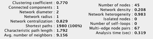
Most common organic layout already inform us about potentially important countries that are highly connected: USA, GBR, FRA, DEU. Layouts based on edge parameters like Biolayout based of bitrade can be even more informative. However, we still do not use actual information about countries.

Organic layout of the imported network of currencies in Cytoscape 3.0. Edge width corresponds to distance, edge colors to bitrade, edge line type to colony variables
So let’s import countries_data.txt through File -> Import -> Table. I check carefully all variables are imported as numerical.
I apply my Cytoscape plug-in DeDaL in order to see the PCA and Elastic Map Layouts.
PCA - principal components analysis
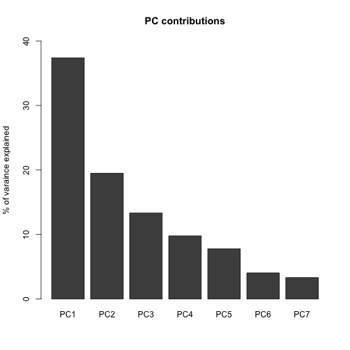
I select Layout -> DeDaL -> Data-driven Layout, to perform PCA without network smoothing and without double centering. A window pops up with percentage of variance explained what can be illustrated with barplot:
Which results in the following layout:

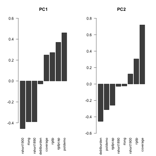
From the PCA we can read that the factors best explaining variance in the data is the level of democracy, market rate (PC1) and coverage & debt (PC2). Therefore, we can see GBP is probably the most important factor. While DEU and FRA are somehow outliers. DEU being the highest in coverage and FRA in democracy index. On the opposite side, there is NZL, AUS and surprisingly CAN & ESP that have big debt. COL, JPN and ICH seem to have high market rate. We can also observe that the countries placed on the right have higher values in bitrade and are the most connected.
Elastic Map - non linear manifolds dimension reduction
It is also possible to perform Elastic Map layout (again no smoothing and no double-centering). A window pops up with information that layout captures 79.19% of variance. In this case Elastic Map layout is quite similar to PCA meaning the problem can be explained in with linear methods.

Networks morphing
Another cool function of DeDaL is network morphing, in this example networks goes from PCA layout to organic layout. Organic layout network is rotated compared to original one to minimize bias due to rotation and mirroring. It is possible to morph any two layouts (i.e. manually created topological layout into organic layout etc.)
Using DeDaL morphing functionality any two networks can be mixed in an interactive way.
Conclusions
From the international currency exchange data, using network approach, we can easily identify countries in the focal point of this dataset. Through PCA, it is possible to identify key variables for analysis of data variability. PCA put in contrast important countries like FRA, DEU and GBR and helps to interpret the differences between them. Therefore, DeDaL provides good and fast insight into the data and allows its visualization, thanks to Cytoscape 3.0 interface no coding sills are needed and graphical proprieties are easily modifiable. It would find the best use combined with domain knowledge and intelligent variable engineering.
Don’t hesitate to download, like and share the tool!
Your imagination is the limit!