Running fastICA with icasso stabilisation

What is fastICA?

Independent Components Analysis (ICA) is a Blind Source Separation (BSS) technique that aims to separate sources maximizing non-gaussianity (or minimising mutual information) of sources and therefore defining independent (or the most independent possible) components.

There exist many different implementations of ICA algorithm: Second Order Blind Identification (SOBI), Hyvarinen’s fixed-point algorithm (FastICA), logistic Infomax (Infomax) and Joint Approximation Diagonalization of Eigenmatrices (JADE).

FastICA (Hyvärinen and Oja 2000) is a popular and fast implementation available in many programming languages.

1. Prewhitenning
   1. Data centering \[ x_{ij} \leftarrow x_{ij} - {\frac {1}{M}}\sum_{j^{\prime }}x_{ij^{\prime }} \] \(x_{ij}\): data point
   2. Whitenning \[ \mathbf {X} \leftarrow \mathbf {E} \mathbf {D} ^{-1/2}\mathbf {E} ^{T}\mathbf {X} \] Where - centered data, is the matrix of eigenvectors, is the diagonal matrix of eigenvalues
2. Single component extraction
   1. Initialize \(w_{i}\) (in random)
   2. \(\mathbf {w}_{i} ^{+}\leftarrow E\left\{\mathbf {X} g(\mathbf {w}_{i} ^{T}\mathbf {X} )^{T}\right\}\mathbf{w}_{i} -E\left\{g'(\mathbf {w}_{i} ^{T}\mathbf {X} )\right\}\)
   3. \(\mathbf{w}_{i} \leftarrow \frac{\mathbf{w}_{i}^+}{\|\mathbf{w}_{i}^+\|}\)
   4. For \(i = 1\), go to step g. Else, continue with step e.
   5. \(\mathbf {w}_{i}^{+} \leftarrow {w}_{i} - \sum_{j=1}^{j-1} {w}_{i}^T{w}_{j}{w}_{j}\)
   6. \(\mathbf{w}_{i} \leftarrow \frac{\mathbf{w}_{i}^+}{\|\mathbf{w}_{i}^+\|}\)
   7. If not converged, go back to step b. Else go back to step a. with \(i = i + 1\) until all components are extracted.

However, the results are not deterministic, as the \(w_{i}\) initial vector of weights is generated at random in the iterations of fastICA. If ICA is run multiple times, one can measure stability of a component. Stability of an independent component, in terms of varying the initial starts of the ICA algorithm, is a measure of internal compactness of a cluster of matched independent components produced in multiple ICA runs for the same dataset and with the same parameter set but with random initialization (Kairov et al. 2017).

What is icasso stabilisation

From (Himberg and Hyvärinen 2003):

We present an explorative visualization method for investigating the relations between estimates from FastICA. The algorithmic and statistical reliability is investigated by running the algorithm many times with different initial values or with differently bootstrapped data sets, respectively. Resulting estimates are compared by visualizing their clustering according to a suitable similarity measure. Reliable estimates correspond to tight clusters, and unreliable ones to points which do not belong to any such cluster

Icasso procedure can be summarized in a few steps:

1. applying multiple runs of ICA with different initializations
2. clustering the resulting components
3. defining the final result as cluster centroids
4. estimating the compactness of the clusters

Icasso stabilisation is implemented in MATLAB. Despite our best effort we did not succeed to replicate this procedure in an open source language.

MSTD measure

In the version of fastica matlab package distributed with deconICA that we named fastica++, contains fasICA algorithm with default parameters, icasso stabilisation and MSTD index calculations and plots.

What is MSTD?

Most stable transcriptome dimension is a metric introduced in (Kairov et al. 2017).

Most Stable Transcriptome Dimension (MSTD) - ranking of independent components based on their stability in multiple ICA computation runs and define a distinguished number of components corresponding to the point of the qualitative change of the stability profile

This measure is not essential for deconICA as in the package we follow strategy of overdecomposition. However, it is useful to know the MSTD that as it is described in (Kairov et al. 2017) to characterize the data and estimate the numbers of components needed for overdecomposition.

Thus, we advise to use the matlab implementation of fastICA fastica++ included in deconICA in order to enjoy the full functionalities of fastICA, icasso and MSTD.

Running fastICA with icasso stabilisation from deconICA

Running matlab from deconICA is very easy. First, if you are not sure if you have matlab, you can run

matlabr::have_matlab()

## [1] TRUE

#it is an example 
library(deconica)
S <- matrix(runif(10000), 500, 5)
A <- matrix(runif(1000), 500, nrow = 5, byrow = FALSE)
X <- data.frame(S %*% A)
res <-
  run_fastica(
    X = X,
    row.center = TRUE,
    n.comp = 5,
    overdecompose = FALSE,
    R = FALSE,
    matlbpth = "/Applications/MATLAB_R2016a.app/bin" #place your path + /bin here
  )

Running fastICA with icasso stabilisation directly in MATLAB

If you want to play with parameters of fastICA or you just prefer to use MATLAB directly, you can use a bunch of functions of deconICA to assure the smooth import of your results.

On an example of simulated matrix with 500 samples and 500 genes.

S <- matrix(runif(10000), 500, 5)
A <- matrix(runif(1000), 500, nrow = 5, byrow = FALSE)
X <- data.frame(S %*% A)
dim(X)

## [1] 500 500

colnames(X) <- paste0("S",1:ncol(X))
row.names(X)<- paste0("gene_", 1:nrow(X))

Yor data need to be centered and duplicated row names should be removed

X.pre <-
  prepare_data_for_ica(X, names = row.names(X), samples = colnames(X))

You can export your data into files saved on your disk.

You can add attribute name if you want to use a different name that the variable name (here ‘X.pre$df.scaled’)

 res.exp <- export_for_ICA(
      df.scaled.t = X.pre$df.scaled,
      names = X.pre$names,
      samples = X.pre$samples,
      n = 5
    )

Then you can run in Matlab

cd 'path to fastica++'

doICA(folder,fn,ncomp)

where

• folder is the path to the folder containing numerical only matrix
• fn is the file name containg the matrix
• n - number of components

here cd './deconica/fastica++'

doICA('/Users/xxxx/Documents/','X.pre$df.scaled_5_numerical.txt',5)

Then, if you followed the steps you can easily import the results.

 res.imp <-
      import_ICA_res(name = "X.pre$df.scaled",
                   ncomp = 5,
                   path_global_1 = "/Users/xxxx/Documents/")

res.imp object has then the fastICA results. You can add additional elements as the initial counts as to any R list object

res.imp$counts <- X

Running fastICA with icasso stabilisation in BIODICA

What is BIODICA

BIODICA is a computational pipeline implemented in Java language for

1. automating deconvolution of large omics datasets with optimization of deconvolution parameters,
2. helping in interpretation of the results of deconvolution application by automated annotation of the components using the best practices,
3. comparing the results of deconvolution of independent datasets for distinguishing reproducible signals, universal and specific for a particular disease/data type or subtype.

BIODICA framework focus is much larger than immune cells. It is quite complete user-friendly software whose applications and functions go beyond scope of this work (see following figure).

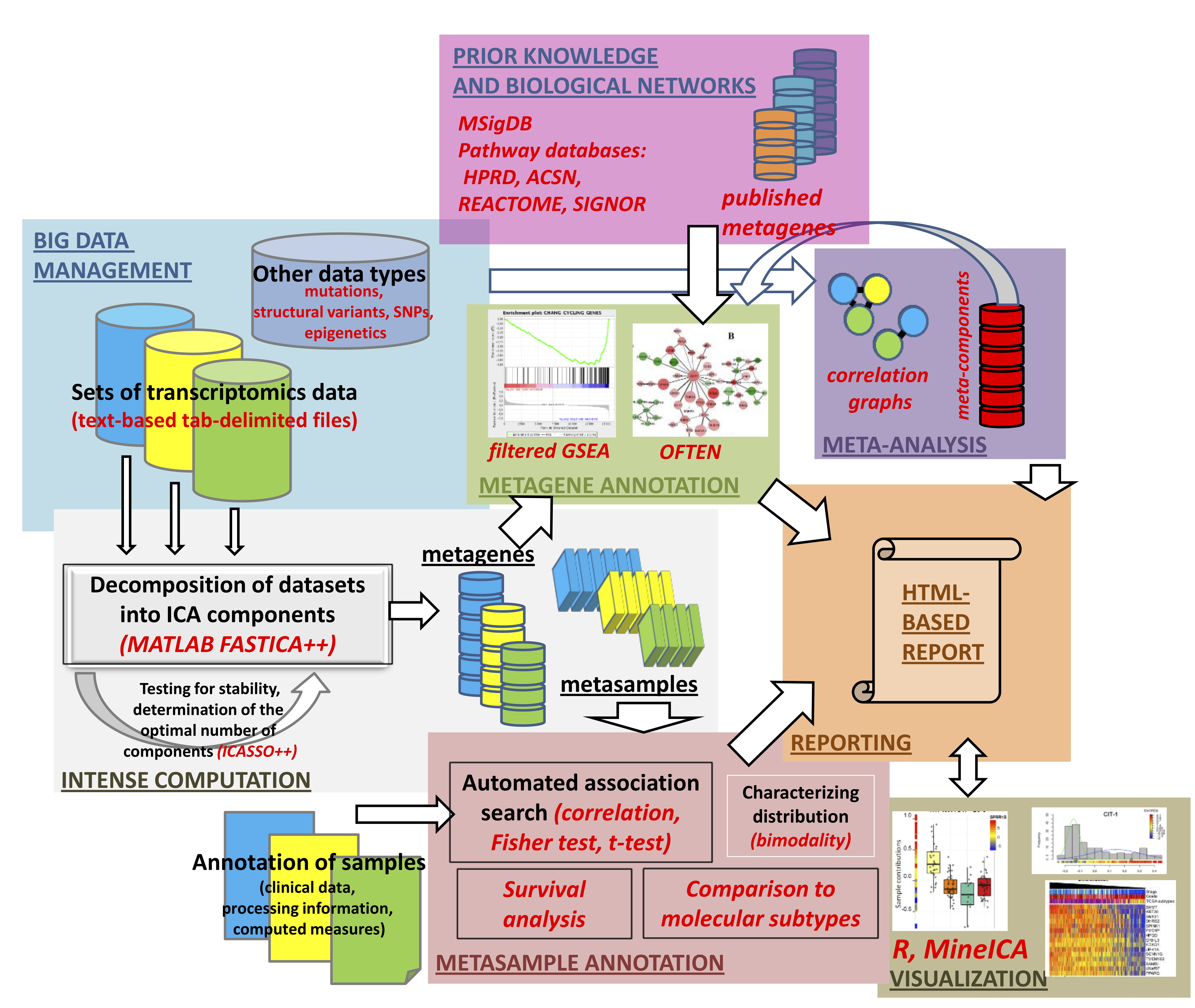
General architecture of the BIODICA data analysis pipeline. Boxes of different colors separates different functional modules of the system. Described functionality corresponds to the BIODICA version 1.0, source: https://github.com/LabBandSB/BIODICA/blob/master/doc/ICA_pipeline_general_description_v0.9.pdf

The full BIODICA tutorial can be found here.

BIODICA is essentially useful for general characterization of signal in transcriptomes.

Using BIODICA

Here we will focus on basic functions as running fastICA.

Requirements:

• Installed Java ver 1.6 or higher
• At least 8Gb of operating memory

In order to run an fastICA decomposition, one can use the GUI interface (see the figure below).

You can launch it by typing (or clicking on the file)

java -jar BIODICA_GUI.jar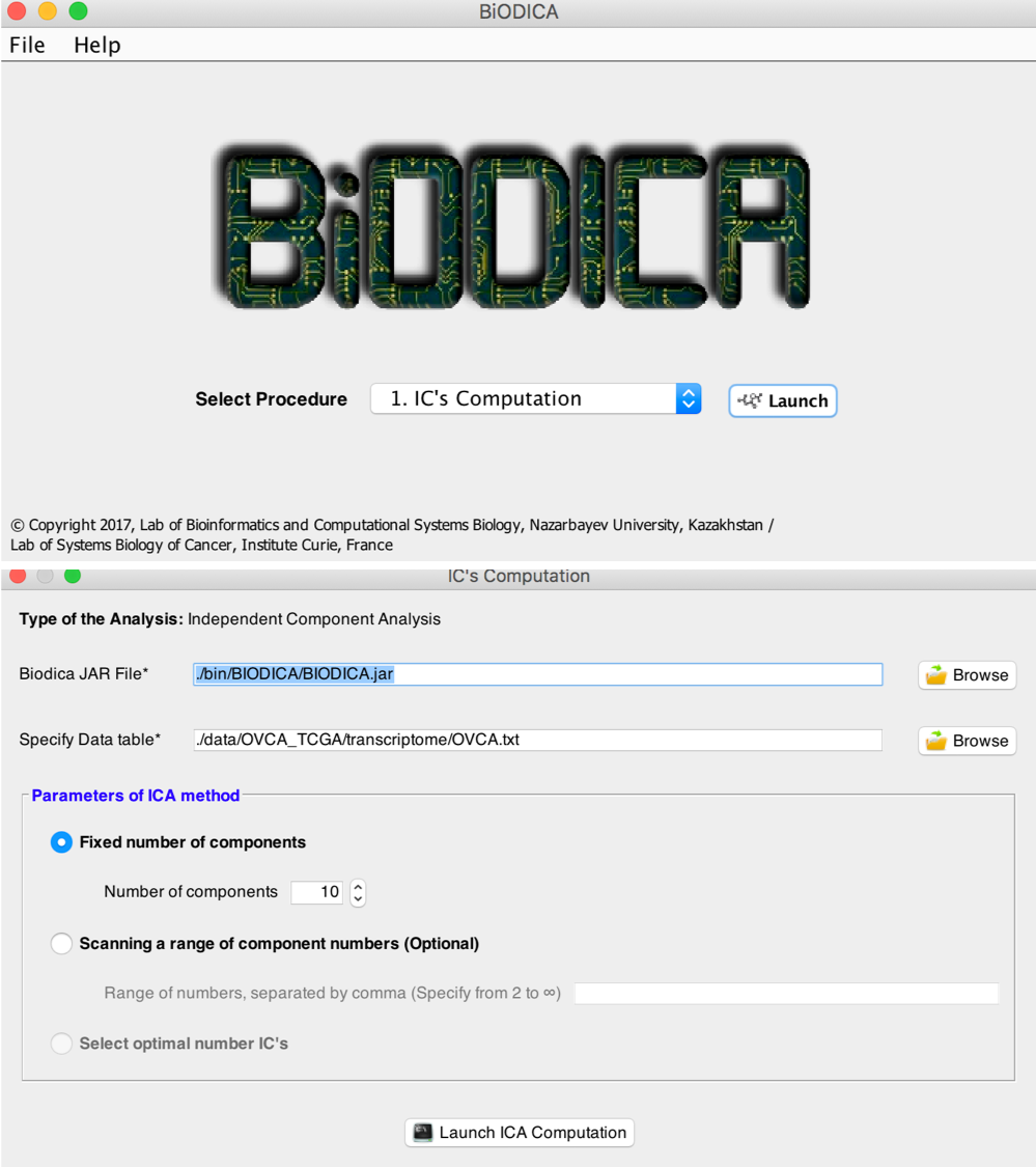

Welcome screen of BIODICA with choice od funcitions and interface of fastICA data and parameters input

It is also possible to run it from command line.

This line will decompose OVCA.txt dataset into 20 components

java -jar BODICA.jar -config C:\Datas\BIODICA\config 
-outputfolder C:\Datas\BIODICA\work\ 
-datatable C:\Datas\BIODICA\data\OVCA_TCGA\transcriptome\OVCA.txt -doicamatlab 20

The input to BIODICA is a dataset with genes in line and samples in columns with sample names and gene names, see sample dataset. However if data is not in log, you need to put in log first. You should also eliminate the duplicated genes (not compulsory but advised for further interpretation). The data will be row centered by default by BIODICA.

Running fastICA with icasso stabilisation in BIODICA docker image

1. Install Docker on your machine
2. Pull the biodica docker image

docker pull auranic/biodica

3. set UseDocker = true in the config file (in your cloned repo).

This procedure is also described on the BIODICA wiki

CONTACTS

All enquires about BIODICA state and development should be sent to

Andrei Zinovyev (http://www.ihes.fr/~zinovyev)

Ulykbek Kairov (https://www.researchgate.net/profile/Ulykbek_Kairov)

BIODICA software

BIODICA - computational pipeline for Independent Component Analysis of BIg Omics Data. It is a collaboration project between Lab of Bioinformatics and Systems Biology (Center for Life Sciences, Nazarbayev University, Kazakhstan) and Computational Systems Biology of Cancer Lab (Institute Curie, France). Principal Investigators and leading researchers of BIODICA Project: Andrei Zinovyev and Ulykbek Kairov.

References

Himberg, Johan, and Aapo Hyvärinen. 2003. “ICASSO: Software for investigating the reliability of ICA estimates by clustering and visualization.” In Neural Networks for Signal Processing - Proceedings of the Ieee Workshop, 2003-Janua:259–68. doi:10.1109/NNSP.2003.1318025.
Hyvärinen, Aapo, and Erkki Oja. 2000. “Independent Component Analysis: Algorithms and Applications.” Neural Networks 13 (45): 411–30. doi:10.1016/S0893-6080(00)00026-5.
Kairov, Ulykbek, Laura Cantini, Alessandro Greco, Askhat Molkenov, Urszula Czerwinska, Emmanuel Barillot, and Andrei Zinovyev. 2017. “Determining the optimal number of independent components for reproducible transcriptomic data analysis.” BMC Genomics 18 (1). doi:10.1186/s12864-017-4112-9.