Chapter 7 Landscape of tumor immunity, with focus on T-cells diversity, uncovered via unsupervised deconvolution applied to bulk transcriptomes across 30 tumor types
Selected content of this chapter is a part of a publication in preparation
7.1 Background
The tumor microenvironment is composed of many different cells including a plethora of immune cells, stromal cells, blood and lymphatic vessels(Galon et al. 2014). The TME compartments’ changes with the cancer type and cancer stage. Recent works showed that immune cells could influence the tumor cells in different ways. The immune therapies take advantage of the protective function of the immune system and aim to activate patients immune defense. FDA has accepted the immune therapies in specific cancer types (Taube et al. 2017). One of the problems of the checkpoint immune therapies is heterogeneity of response rate, which can vary, i.e., from 10–40% in the case of PD-L1 blocking (Zou, Wolchok, and Chen 2016). To respond to this challenge, a better understanding of the role of immune cells in cancer is necessary.
A link between patients response to the therapy and the presence of tumor-infiltrating lymphocytes (TILs) was identified (Topalian et al. 2016). T cells differentiate into highly diverse subsets expressing unique markers depending on their environment (Wong et al. 2016). Suppressive nature characterizes the infiltrating regulatory T cells (or Tregs) from colon, lung, and breast cancers in transcriptomic studies (De Simone et al. 2016; Plitas et al. 2016). The primary objective of the checkpoint therapies is to activate CD8+ cytotoxic T cells in the tumor microenvironment. CD8+ T cells can be impaired by suppressive T regs or exhausted due to a unique transcriptional state (Chen and Mellman 2017). A better understanding of T cells heterogeneity and functions can significantly advance the immune checkpoint therapies.
Nowadays, research generates a massive amount of data on TME. Many experiments requiring fresh samples are costly and time-consuming. On the other hand, there is available a vast collection of public data that are not always fully exploit. An example is bulk transcriptome data in which, for the heterogeneous samples like PBMC and tumor biopsies, the expression profiles of distinct cell types are mixed in each sample. Several methods were proposed to estimate abundance of immune infiltration in cancers (Becht et al. 2016; Newman et al. 2015; Aran, Hu, and Butte 2017; Racle et al. 2017). However, they do not propose simultaneous estimation of infiltration abundance and context-specific signatures of the immune cell types. Different approaches (i.e., clustering (Chifman et al. 2016), attractor metagenes (Cheng, Yang, and Anastassiou 2013), differential gene expression (Cieślik and Chinnaiyan 2017)) were adapted to discover signatures that would describe cancer transcriptomes.
In this work, I propose an unsupervised deconvolution approach that applied to bulk cancer transcriptomes can detect cell-type specific signals and cellular programs. In contrast to previously published complete deconvolution approaches applied to PBMC (Repsilber et al. 2010; Gaujoux and Seoighe 2012)or yeast cell-cycle (Wang et al. 2016), using DeconICA R package (Czerwinska 2018), I performed pan-cancer tumor transcriptome deconvolution of 119 datasets across 30 tumor types. Also, I dedicated an extra effort to describe T-cell diversity in deconvoluted cancers types. Besides, I apply DeconICA deconvolution to five single-cell datasets to integrate them and compare with created decomposed bulk transcriptome landscape.
7.2 Results
7.2.1 Unsupervised deconvolution of 119 datasets
In this study, we collected 119 datasets with a total of 26561 samples across 30 tumor types (Fig 7.1. Data were collected from public repositories (GEO, ArrayExpress). If normal samples were present in the dataset, they were excluded before running the analysis. The common cancer type we analyzed was the lung cancer (18 datasets), followed by colorectal (11 datasets) and breast cancer (9 datasets). Each dataset was analyzed independently with DeconICA R package using stabilized ICA (see methods). The primary output of the DeconICA pipeline for each dataset was a set of independent components, to which I will also refer as metagenes, which are weighted list of genes. The positive end of a metagene represents a characteristic transcriptomic signature that can be interpreted in terms of cellular processes, state or cell type. The second output of the DeconICA pipeline was the abundance scores of each interpreted component across samples.
Figure 7.1: Count of the datasets analyzed with DeconICA. Datasets (Supplementary tab. 7.1) were counted depending on the cancer type. The most frequent analyzed cancer type was lung cancer.
7.2.2 Interpretation of the immune components
The filtered correlation network (Fig. 7.2) shows a presence of communities of metagenes which can be interpreted based on the higher ranked genes. In our analysis, each metagene was labeled based on its correlation with reference profiles which are either metagenes obtained from previous pan-cancer studies (Biton et al. 2014) or optimized for deconvolution (Newman et al. 2015) integrated into the DeconICA R package. For each dataset and HTML report was generated (see supplementary) to summarize the analysis. To best visualize the data in the 2D space, I used the UMAP dimension-reduction algorithm based on correlation distance. I selected the parameters to best separate the clusters of different component types, for visualizations with the tSNE algorithm and different UMAP parameter settings see supplementary figures 7.10 and 7.11. Based on the distance from the median and manual curation, I eliminated susceptible mislabelled components which resulted in the clearly defined landscape of tumor signals (Fig. 7.3). One can observe, compact clusters of identified signals, including 13 cell types (B cells, T cells, Dendritic cells, Eosinophils, Macrophages (M0, M1,M2), Mast cells, Monocytes, Neutrophils, NK cells, Plasma cells, Myofibroblasts/CAFs), 6 general signals (Cell cycle, Stress, GC content, Smooth muscle, Mitochondria translation, Interferon), 2 cancer-specific signals (basal-like subtype of breast cancer, BLCA pathways and Urothelial differentiation of bladder cancer) and general immune signals. To confirm the labeling, I visualized the known cell type markers on the 2D landscape for T cells, B cells, Myeloid cells and CAFs (Fig. 7.4). It can be observed that the cell-type markers are highly expressed in the area labeled as expected cell types.
Figure 7.2: Correlation graph of metagenes. RBH network as described in (Cantini, Kairov, et al. 2018) represents reciprocal correlations between vectors of metagenes. Each point here is a metagene. Point colors correspond to the cancer type. Only reciprocal correlations were kept and with absolute Pearson correlation >0.2. The squares defining functional territories were added manually based on the top genes and correlation with the reference metagenes. Only selected processes/cell types were depicted.
Figure 7.3: 2D representation of labeled metagenes using UMAP dimension reduction with correlation distance as metric. UMAP was run on all labeled components from bulk transcriptomes (parameters specified in Methods. The outliers were removed as described in Methods. Each point is a metagene (ICA component). Colors correspond to the attributed labels. The distance between points is a non-linear function of the metagenes proximity.
Figure 7.4: Cell markers expression in the metagenes of T cells, B cells, Myeloid cells and CAFs. Known cellular markers were used to confirm labeling of the metagenes. Color scale corresponds to the weight of the gene in the immune components with red for high weights and blue for low weights (see legend). The squares around metagenes delimit approximatively the area of the labels attributed by DeconICA (Fig. 7.3)
7.2.3 Quality of cell-type signal extraction is affected by tumor type
As the signal extraction is purely data-driven, it is not guaranteed to extract cell-type signals from all datasets (Fig. 7.5). It can be observed that in nearly all datasets at least one component related to the myeloid cells (macrophages, monocytes, eosinophils, neutrophils) was identified and in many multiple components corresponding to the cell types. For B cells (labeled Plasma cells or B cells) usually, one component is identified. Finally, the T-cell/NK component was identified in most of the datasets but with less success rate than the aforementioned immune cells (T cells and NK were regrouped because in most cases, the unsupervised analysis cannot differentiate these profiles).
One factor that affects the quality of the decomposition is the number of samples. This is why I analyzed datasets containing more than 60 samples with preference to large cohort studies. However, some other factors seem to affect the quality of the decomposition. I observed the average correlation with the reference profile for T cells, B cells and Myeloid cells (Fig. 7.6). It can be observed that AML has a remarkably high correlation with the reference cell types. Besides, breast cancer has a quite good correlation (always in the top 3). Lung cancer is usually placed in the middle. Colorectal cancer has a lower correlation for T cells than for B cells and Myeloid cells. It can also be observed that in some cancer types, some immune cells were not detected (Supplementary fig. 7.12). For instance, in multiple myeloma only T cells were detected, in the bladder, glioma, gastric, pancreas, THYM, uterine, colon adenocarcinoma, rectum, testicular, some soft tissue sarcomas no T cells were detected. In the breast, HNSCC, prostate, Ewing, stomach and other cancers all three cell types were detected.
Figure 7.5: Detection count of immune cells in analyzed datasets. In each of the analyzed datasets (rows), the number of detected components with a given label (columns) was counted. Values for each immune cell type were reported, and cumulative count for T cells and NK cells, B cells, and Plasma cells, and all type of Myeloid cells summed were reported as well (in blue). Color code distinguishes tumor types (see legend). The black color of the heatmap cell indicates no component detected. Myeloid and B cell components were detected in almost all datasets, while the T cell/NK component only is a part of the data.
Figure 7.6: Correlation of cell-type metagenes with the reference profiles of T cells (A), B cells/Plasma (B), Myeloid cells (C). For the three cell types, average correlation per tumor type was computed. Tumor types were ordered in ascending order.
7.2.4 Deconvoluted bulk transcriptome T cell signatures showcase different cell states in cancers
Then, I focused on the components labeled as T cell. The genes present in all T cell components were ranked based on the frequency they are present in the components. Among top one hundred genes (Supplementary table 7.7, there are classical T-cell markers: CD3D, cD8A, CD2, CD52 and well as chemokines and GZMK, GZMB, interleukins (IL2) and receptors (IL7R, KLRB1). Some of these molecules are specific to T cell, and some other shared between cytotoxic T cells and NK cells, different ones can characterize all leucocytes.
To better understand possible T cell signatures diversity in different cancers, I used PCA projection. PCA axes can be interpreted through the loadings which enable to define variables (genes) that contribute the most to the direction. I considered the top 100 genes for the positive and negative sides of PC1 and PC2 for the interpretation with online enrichment tool Enrichr (Chen et al. 2013). The top ten genes of each side of PC1 and PC2 can be seen in the Supplementary tables 7.3-7.6. I divided components into three groups based on possible interpretation of the t-cells states (Fig. 7.7C). Cytotoxic phenotype, leucocytes activation characterize the group 1 (associated with the negative part of the PC1). Among this “activated T cell,” signatures are components extracted from DLBC, colorectal cancer, glioma, gastric, ovarian cancers (Fig. 7.7B). The positive part of PC1 does not seem to reflect any strong cell state, containing a lot of small nucleolar RNAs, with enrichment in cofactor activation of translation, fatty acid oxidation and mTORC1 which role is active translation and protein production. The interpretation of the cells in groups 2 and 3 makes more sense along the PC2 axis. The signature of the PC2 positive side seems to be related to chemokine production and B-cell characteristic markers CD79. The group 2 components were mostly extracted from lung, colorectal and breast cancers. The group 3 (negative loading of PC2), is associated with high migration, cytokines, and NK-like activity: GZMA, NKG7 and also INFG. The signatures from the group 3 were mostly obtained from DLBCL, liposarcoma, melanoma, kidney. Besides, I tempted to identify the cells with a collection of T-cell related pathways (with many pathways related to T helpers activity) (courtesy of the team of Vassili Soumelis). From the GSVA (Hänzelmann, Castelo, and Guinney 2013) scores, the group 3 has the highest enrichment in the CD8 signature, INF response. The group 2 seem to have some CD4 regulatory pathways activated and type II INF response. The group 1 is negatively enriched in most of the pathways except “Tosolini.Th2.signature”. An observation can be made on the how insightful are distinct signatures. Many redundant pathways indicate different enrichment scores which do not help in the interpretation.
Figure 7.7: Analysis of T cell diversity. The T cell labeled components from bulk transcriptomes were projected in PC1 and PC2 space. The components were coloured by tumor type (B) (see legend) and groups (C) defined by PCA coordinates: group 1: PC1\(^-\), group 2 PC1\(^+\) & PC2\(^+\), group 3 PC1\(^+\) & PC2\(^-\). The GSVA enrichment scores of T cell pathways were plotted in the heatmap. Cancer types and groups were signaled with a color code (see legend).
7.2.5 Single-cell RNAseq deconvolution leads to cell-specific metagenes
In addition to deconvolution of bulk transcriptomes, I used five public datasets of single-cell RNA-seq of human cancers (Breast, CRC, Melanoma, Liver, Head and Neck). The datasets sources and precise count of sequenced cell types (labels attributed by authors) can be found in Supplementary table 7.2. Only malignant cells were used in the analysis. First, the raw count data were knn-smoothed (Wagner, Yan, and Yanai 2018) to palliate the drop-out effect of scRNA-seq. Then DeconICA was used to first, find MSTD(Kairov et al. 2017), then each dataset was decomposed to its optimal dimension. Cell-type specific components were identified through correlation with the reference profiles and double-confirmed through authors labels (Supplementary fig. 7.13). I detected T cells, B cells and Myeloid cells in all five datasets and their Pearson correlation coefficient with reference T-cell profile around 0.6, Myeloid 0.4 and B-cells variable (0.2-0.6). Besides detecting cell-type specific signals, I also observed cell-cycle, mitochondria translation, interferon, and stress. The extracted metagenes were plotted together with the bulk metagenes in a 2D UMAP plot (Fig. 7.8A). The single cell components incorporate correctly in the previously established bulk transcriptome landscape. To verify if there can be defined a closer relationship between T cell components (single cell and bulk) from the same cancer type, I computed Pearson correlation between the components (7.8B). The results indicate that single cell components are strongly correlated with each other (especially CRC, Breast, and HNSCC). There is a group of components that is higher correlated with the single cell signatures. This group corresponds to previously described groups 2 and 3, where most of the components of the group 3 (that was mostly obtained from CRC and liver) are highly associated with CRC single cell components. Therefore a strong association between cancer T cell components can be observed even though it is not exclusive (B cell bulk components correlate well with CRC, Breast, and HNSCC) and single cell extracted components correlate with components originating from diverse tumor type.
Figure 7.8: Metagenes from the single cell and bulk transcriptome (A) The components extracted from five single-cell datasets were depicted together with bulk components. Most of the scRNA-seq-derived components integrate well with the established space in proximity to medians of bulk components for cell types or cellular programs. Shapes correspond to data type, colors to label or cancer type (see legend). (B) T cell components from extracted from single cell datasets and bulk datasets were correlated. The single-cell T cell signatures of CRC, Breast, and HNSCC are strongly correlated together. They also correlate with bulk T cell signatures, mostly with previously defined groups 2 and 3.
7.2.6 Landscape of patient based on the immune infiltration scores
Besides, I computed abundance scores using DeconICA R package for all signals identified in the analysis. I used the 2D UMAP euclidean distance plot to visualize the patient landscape. It can be observed that most of the samples from the same dataset cluster together. There is an unusual cluster of patients of different cancer types including ovarian, pancreas, breast and lung cancer samples. It is not trivial to interpret the cluster repartition of the sample space given the number of samples. This landscape should be interpreted together with patient survival data to establish a link between the clusters and survival. The analysis of the sample space as part of this work is still unfinished.
Figure 7.9: Patients landscape based on the signal abundance scores The abundance scores for each detected component were computed with DeconICA. The UMAP 2D representation using Euclidean distance (see Methods). Most of the samples cluster by data set. Some (lung) cluster by tumor type. Some datasets are on the opposite sides of the plot (BRCA).
7.3 Discussion
In this work, I performed an unsupervised deconvolution of 26561 samples across 30 cancer types. First, to our knowledge it is one of the largest metanalyses of cancer transcriptomes. Recently published works (Thorsson et al. 2018; Tamborero et al. 2018) were limited to TCGA data (10 000 samples). In this analysis, unlike the studies mentioned above, we compare information extracted from cohorts that were generated and processes in different projects. By doing this, I challenged the possible biases of data processing and technologies as well us unknown factors affecting the data sources.
Secondly, (Newman et al. 2015; Racle et al. 2017; Aran, Hu, and Butte 2017; Becht et al. 2016) and others proposed digital deconvolution of cancer transcriptomes. However, their methods are based on pre-defined reference profiles for which abundance is estimated in the cancer samples. In contrast, we proposed a way to discover the factors governing the samples directly from the data. Our method, provide not only the abundance scores of immune cell and other signals but also the signatures of those factors: metagenes. In this work, I compared the metagene signatures between tumor types. This analysis cannot be done using supervised deconvolution algorithms. Unsupervised cell-type deconvolution algorithms (Newberg et al. 2018; Ogundijo and Wang 2017; Wang et al. 2016; Repsilber et al. 2010) were never applied in the cancer context, other works (Moffitt et al. 2015; Brunet et al. 2004; Biton et al. 2014) did not show cell-type level resolution of signal deconvolution.
Using marker genes and dimension reduction, I validated my labeling to represent bona fide immune cells, other cell types (i.e., CAFs) and cellular processes (cell cycle, stress, translation). Also, using clusters obtained from 2D dimension reduction correlation based UMAP, I removed possible mislabelled components. The labeling process should be improved in the future to decrease the false positive rate.
I proved the utility of the ICA deconvolution applied to the single cell data of tumor transcriptomes. The ability of matrix factorization to extract cell-specific and ‘cellular activity’ signatures was previously demonstrated using NMF in (Kotliar et al., n.d.). To my knowledge, no one showed a similar capacity of ICA. My cell-specific signal extraction was confirmed with cell type labels given independently by article authors. Cell type signals were found without error except for NK/T cell mixed signal in Head and Neck cancer. However, no NK cells were labeled by authors. Also, the decomposition of Liver cancer T cell is quite astonishing. ICA was unable to distinguish cytotoxic T cells (TC) from T cell helpers (TH) or T reg (TR). The reason may be that normalized by authors data were directly used, maybe data transformation destroyed part of the variability (Paulson et al. 2017). Another possibility is that the is not enough variability in the data of T cells only to perform an unsupervised deconvolution. I was still able to identify cell cycle and interferon profiles. Besides 4 of ICA components corresponded closely (0.69-0.75 Pearson correlation coefficient) to an average of clusters discovered by authors (Zheng et al. 2017).
I observed detection limits of unsupervised deconvolution, indicating that in some tumor types it is more challenging to extract T cells or B cells. Another observation was that for the extracted components, the average correlation is different depending on the cancer type. One explanation of high correlation of AML with reference profiles is that the samples are liquid, AML is a blood cell cancer in bone marrow, and deconvolution of liquid samples (blood or bone marrow samples) is less challenging than solid samples Racle et al. (2017). However, in this case, we would expect high correlation coefficients for DLBCL which are biopsied of lymph nodes. Another possible reason is that the signal of healthy immune cells is mixed with the malignant immune cells increasing the signal strength. However, the reason for breast cancer to have components highly correlating with the reference is more mysterious. Tamborero et al. (2018) (Fig. 4) discussed three possible scenarios of the impact of the immune infiltrate on cancer: cytotoxic infiltrate, suppressive infiltrate and poorly cytotoxic infiltrate. Breast cancer is characterized mostly by cytotoxic infiltrate it is possible that the highly cytotoxic signal is strongly expressed in the transcriptome and therefore detectable from the bulk. According to another pan-cancer study of Thorsson et al. (2018), highest leucocyte fraction can be found in lung, pancreatic, HNSC and testis cancers. It is essential to add the immune infiltration fractions in (Thorsson et al. 2018) was evaluated using CIBERSORT (Newman et al. 2015).
From the technical side, in smaller datasets, I was usually not able to detect cell-type components, and one immune component was found. This generic immune component “M6_IMMUNE” was the one correlating best with B cells, T cells, and Myeloid cells. Among our labels, I also identify ‘Immune’ components that were the components correlated with the immune signal but to which no label could be attributed.
T cell diversity analysis leaves some unanswered questions. Recent works demonstrated essential differences between blood and cancer T cell profiles (Schelker et al. 2017; Tirosh et al. 2016). I tempted to interpret the diversity of T cells using unsupervised (PCA) and supervised strategy (GSVA). The three groups I could define correspond to activated T cells (group 1), Tumor killing and migrating T cells (group 3) and generic leucocyte (group 2). In (Thorsson et al. 2018) the role of INFG (found enriched in group 3 of deconvoluted T cell signatures) is linked with their INFG-dominant and Inflammatory clusters. The enrichment analysis (GSVA) did not help much to describe the groups better. It was shown that not all signatures are well-adapted to transcriptome analysis (Cantini, Calzone, et al. 2018). From GSVA results, a hypothesis can be made that the group 2 may represent the immunosuppressed T cells, but there is a lack of direct evidence.
I fused in the same pan-cancer landscape signatures derived from bulk transcriptomes and scRNA-seq. The single-cell derived signatures incorporated well into the established immune landscape. Previously (Schelker et al. 2017; Racle et al. 2017; Görtler et al. 2018) proposed to use single-cell derived signatures to improve the deconvolution performance. So far, single-cell signatures for all cancer types are not available. In my study, ICA derived scRNA-seq signatures for T cells are closely correlated with each other. It may indicate a bias related to the data type (Kharchenko, Silberstein, and Scadden 2014). It can also be related to the quality of the signal that should have much less noise (as each sample represents one cell) than in bulk tumors. This result does not allow to conclude if the single cell signatures should be used as a reference in the future works. Furthermore, for the T cell signature from the bulk, one would expect the highest correlation between the same cancer type. The correlation between cancer type bulk and single-cell components are high but not for all the components. Especially, former called group 1 of cells seem to be very weakly correlated with the single cell T cell signatures. This can be of technical matter (noisy components) or biological matter (different cell state). The number of scRNA-seq tumor data increases exponentially, and hopefully, soon, it will be possible use more cancer types and confront different single-cell datasets of the same tumor to acknowledge possible technical biases and include higher patient heterogeneity (Svensson, Vento-Tormo, and Teichmann 2018).
Finally, the abundance scores were used to compose a landscape of samples. Previous pan-cancer work (Tamborero et al. 2018, Fig 1D) applied to TCGA data showed different effect of immune infiltration on patient survival that has a good impact on most of the cancer types (including BRCA, LUAD, SKCLA, ACC), and negative impact in LGG, UVM and seem to have neutral impact for instance for STAD, GBM, ESCA, KIRC, KIP, THCA, OV. As it is a part of the ongoing analysis, no conclusions can be made for our results, and it will be stated in an analysis of cancer datasets beyond TCGA previous findings are confirmed. Also, there is potential to find patient clusters, inter tumor type that would be due to unique features related to patient survival.
7.4 Conclusions
In this work, I performed a proof of concept of pan-cancer unsupervised deconvolution. I demonstrated that the ICA-based components extracted from bulk transcriptomes correspond to the immune cell-type signals. I also integrated cell type-specific signatures form single cell tumor data. In addition, I identified, in both bulk and single cell, set of cellular programs deconvoluted from the cell-type signatures. I discussed the limits of unsupervised deconvolution and possible reasons for the difference in the quality of deconvolution that is related to the tumor type. I also analyzed the T cells diversity with a discovery of three groups of T cell states. At last, I generated samples landscape based on the abundance scores obtained thanks to the top genes of the discovered independent components.
Shortly, the analysis will continue in order to characterize the T cell groups better. A similar analysis can be performed to study other cell types. There is also a possibility to study the impact of the cell cycle (proliferation) on the cell type-specific signatures. In addition, the sample landscape should be explained. Finally, the findings of this study should like to cancer subtyping and patients survival to fully exploit its potential in translational research direction.
In a longer perspective, the transcriptome landscape could be completed by the whole exome, genomic and epigenetic data to gather information about driving mutations, transcription factors, neoantigens and TCR/BCR diversity patterns
7.5 Methods
7.5.1 Data sources
All data were collected from public repositories TCGA (Weinstein et al. 2013), GEO (Edgar, Domrachev, and Lash 2002) and Array Express (Kolesnikov et al. 2015). The datasets were filtered based on the number of samples (min 60) and missing value ratio. The detailed list of bulk transcriptome datasets used in this study, with the number of samples, number of probes, technology, reference, and number of dimension after DeconICA analysis can be found in the Supplementary table 7.1. The single cell data were accessed from original publications as listed in Supplementary table 7.2. The original cell type labels were used as published by authors (the labels for Breast cancer (Chung et al. 2017) were provided through private communication with authors).
7.5.2 Data pre-processing
The bulk transcriptome data normalized by authors were used in this study. First, if normal tissue samples were present, they were excluded from the analysis. Then probe names were converted to HUGO names using Bioconductor Biomart R package (Baker 2012; Durinck et al. 2009). Then DeconICA R package (Czerwinska 2018) was applied to analyze the data. DeconICA at first excludes repeated gene names keeping the most variant genes; then data are transformed into \(log_2(x+1)\) and row centered. The number of the components is selected automatically in overdecomposition mode to either to 100 or number of PCA components explaining 90% of variability (see the R package documentation for more details).
The single cell data in the first place were treated with knn-smoothing algorithm (Wagner, Yan, and Yanai 2018); Python implementation published on github to minimize the drop-out effect. Then the probe names were converted into HUGO symbols; duplicated entries remove, then data were transformed by DeconICA R package just like described above. The main difference was the number of dimension with was set according to the MSTD dimension computed with “batchICA” function of the fastICA toolbox.
7.5.3 Data analysis
7.5.3.1 ICA deconvolution
Prepared data matrices are passed to fastICA MATLAB with icasso stabilization (see this for more details) distributed with BIODICA tool. The transcriptomes were therefore decomposed to a set of metagenes (\(S\) matrix) and metasamples (\(A\) matrix). In this work, I used metagenes that are weighted gene vectors.
7.5.3.2 Correlation plot
The reciprocal correlation plot was obtained with RBH function in BIODICA tool and visualized in Cytoscape 2.0 (Shannon et al. 2003).
7.5.3.3 Labelling the components
Using integrated into DeconICA reference profiles of 22 immune cells from (Newman et al. 2015) and reference metagenes from (Biton et al. 2014) immune components were interpreted. An HTML report was generated for each dataset, and all of the reports can be accessed here. The labels were attributed though reciprocal correlation for reference metagenes and maximal correlation for cell type profiles. Only labeled components were retained for further analysis to facilitate data storage and management (reduction from ~120000 components to ~1900 labeled components).
7.5.3.4 Missing values imputation
The retained components were merged on gene base, and missing values were imputed using probabilistic principal components analysis (“ppca” in pcaMethods Bioconductor R package (Stacklies et al. 2007) adapted from (Porta, Verbeek, and Kröse 2005)) and k-Nearest Neighbour algorithm (imputation package by Jeffrey Wong (Cai, Candès, and Shen 2008; Troyanskaya et al. 2001)). The correlation of the data with the imputed values for both methods was 99.7%. Therefore ppca-based was retained as it was significantly faster.
7.5.3.5 Visualization of the data in the 2D space
Among algorithms commonly used for dimension reduction and visualization such as PCA, ISOMAPS, tSNE (Van Der Maaten and Hinton 2008), I chose a new one named UMAP (Mcinnes and Healy 2018): Uniform Manifold Approximation and Projection for Dimension Reduction that is based on Laplacian eigenmaps, highly scalable, reproducible. It was recently applied to biological data (Becht et al. 2018). The advantage of using UMAP is the possibility to chose the distance metric and control different parameters (min distance, number of neighbors). Also, empirically, UMAP provided the best separation of labeled components in clusters (Supplementary fig. umap and tsne). UMAP Python implementation published on github was used in this work. The choice of parameters (n_neighbors=20, n_components= 2, min_dist=0.05, metric=“correlation”) for UMAP was based on Hopkins statistic (Hopkins 1954) (the mean nearest neighbor distance in the random dataset divided by the sum of the mean nearest neighbor distances in the real and across the simulated data set).
7.5.3.6 Elimination of false positives
To exclude false positives median was computed for each group of components labeled in the same way. The medians were plotted together with the single components using UMAP with the same parameters as mentioned above. Any points located in UMAP 2 dimensions further from the median group component than two standard deviations were removed from the plot. Remaining components were used for further data analysis.
7.5.3.7 T-cells heterogeneity
The T-cell components were selected from the labelled components and PCA (R function “prcomp” with parameters center = TRUE, .scale= FALSE). The loadings were extracted from the prcomp object “$rotation”. The top genes of PC1/PC2 negative and positive side interpretation were performed with Enrichr (Chen et al. 2013). The enrichment with the T cell pathways (available under request) was computed using the GSVA algorithm (Hänzelmann, Castelo, and Guinney 2013), implemented in the GSVA R package.
7.5.3.8 Single cell data
The single cells datasets were analyzed with DeconICA. The cell-specific components were identified. Abundance scores were computed with arithmetic mean of top 10 genes. The density of the abundance was plotted against the cell type labels (Supplementary fig. 7.13). The labeled components were merged with the labeled components from the bulk data, and the missing values were imputed using ‘ppca’ as described above. The T-cell single cell signatures were correlated with the bulk T-cell signatures using Pearson correlation. Results were visualized as a heatmap (R package pheatmap).
7.5.3.9 Sample landscape
In each dataset abundance scores were computed based on the top 10 genes, then the score for each cell type was mean centered. The abundance scores were merged based on labels. For missing labels, 0 abundance value was reported. UMAP with Euclidean distance was used to project the sample landscape in 2D (parameters: n_neighbors=20, n_components= 2, min_dist=0.4, metric=“euclidean”).
7.5.4 Software
Data were manipulated and visualized using ggplot2 (Wickham 2016), pheatmap(Kolde 2018), gridExtra(Auguie 2017), lattice(Sarkar 2008), plotly(Sievert et al. 2017), deconica (Czerwinska 2018) R packages. R version 3.5.0. R studio version 1.1.447.
R version 3.5.0 (2018-04-23)
Platform: x86_64-apple-darwin15.6.0 (64-bit)
Running under: macOS High Sierra 10.13.5

Matrix products: default
BLAS: /System/Library/Frameworks/Accelerate.framework/Versions/
A/Frameworks/vecLib.framework/Versions/A/libBLAS.dylib
LAPACK: /Library/Frameworks/R.framework/Versions/3.5/Resources/lib/libRlapack.dylib

locale:
[1] en_US.UTF-8/en_US.UTF-8/en_US.UTF-8/C/en_US.UTF-8/en_US.UTF-8

attached base packages:
[1] parallel  stats     graphics  grDevices utils     datasets  methods   base

other attached packages:
 [1] randomcoloR_1.1.0   corrplot_0.84       Hmisc_4.1-1         Formula_1.2-3
 [5] survival_2.42-3     lattice_0.20-35     GGally_1.4.0        plotly_4.7.1
 [9] bindrcpp_0.2.2      dplyr_0.7.6         ggpubr_0.1.6        magrittr_1.5
[13] ggplot2_3.0.0       pcaMethods_1.72.0   Biobase_2.40.0      BiocGenerics_0.26.0
[17] biomaRt_2.36.1

loaded via a namespace (and not attached):
 [1] bitops_1.0-6         bit64_0.9-7          RColorBrewer_1.1-2
 [4] progress_1.2.0       httr_1.3.1           rprojroot_1.3-2
 [7] tools_3.5.0          backports_1.1.2      R6_2.2.2
[10] rpart_4.1-13         DBI_1.0.0            lazyeval_0.2.1
[13] colorspace_1.3-2     nnet_7.3-12          withr_2.1.2
[16] tidyselect_0.2.4     gridExtra_2.3        prettyunits_1.0.2
[19] bit_1.1-12           curl_3.2             compiler_3.5.0
[22] htmlTable_1.11.2     labeling_0.3         scales_0.5.0
[25] checkmate_1.8.5      stringr_1.3.1        digest_0.6.15
[28] foreign_0.8-70       rmarkdown_1.10       base64enc_0.1-3
[31] pkgconfig_2.0.1      htmltools_0.3.6      htmlwidgets_1.2
[34] rlang_0.2.0.9001     rstudioapi_0.7       RSQLite_2.1.1
[37] shiny_1.0.5          bindr_0.1.1          jsonlite_1.5
[40] deconica_0.1.1       crosstalk_1.0.0      acepack_1.4.1
[43] RCurl_1.95-4.10      Matrix_1.2-14        Rcpp_0.12.17
[46] munsell_0.5.0        S4Vectors_0.18.1     stringi_1.2.2
[49] yaml_2.1.19          Rtsne_0.13           plyr_1.8.4
[52] grid_3.5.0           blob_1.1.1           promises_1.0.1
[55] crayon_1.3.4         cowplot_0.9.2        splines_3.5.0
[58] hms_0.4.2            knitr_1.20           pillar_1.2.2
[61] stats4_3.5.0         XML_3.98-1.11        glue_1.2.0
[64] evaluate_0.10.1      V8_1.5               latticeExtra_0.6-28
[67] data.table_1.11.2    httpuv_1.4.3         gtable_0.2.0
[70] purrr_0.2.4          tidyr_0.8.1          reshape_0.8.7
[73] assertthat_0.2.0     mime_0.5             xtable_1.8-2
[76] later_0.7.2          viridisLite_0.3.0    tibble_1.4.2
[79] pheatmap_1.0.10      AnnotationDbi_1.42.1 memoise_1.1.0
[82] IRanges_2.14.8       cluster_2.0.7-1
ICA computation was performed with fastICA (fastica++) (distributed with BIODICA ) toolbox in MATLAB_R2016a.
7.5.5 Hardware
All computations were performed on MacOS High Sierra version 10.13.5.
7.6 Supplementary
7.6.1 Figures
Figure 7.10: Metagenes 2D tSNE landscape, parameters testing. 2D visualization with tSNE was tested with different perplexity parameters. The component types in the middle of the plot are not well separated.
Figure 7.11: Metagenes 2D UMAP landscape, parameters testing. 2D visualization with UMAP was tested with nearest neighbors parameters. For all parameters, clusters of components are well defined.
Figure 7.12: Ratio of detected components by cancer type. From the Fig. 7.5 data were regrouped by cancer type, and a ratio of the number of components over the number of datasets was reported. Values for each immune cell type were reported, and cumulative count for T cells and NK cells, B cells, and Plasma cells, and all type of Myeloid cells summed were reported as well (in blue). Color code distinguishes tumor types (see legend). Black color indicates no component detected. Myeloid and B cell components were detected in almost all datasets, while the T cell/NK component only is a part of the data.
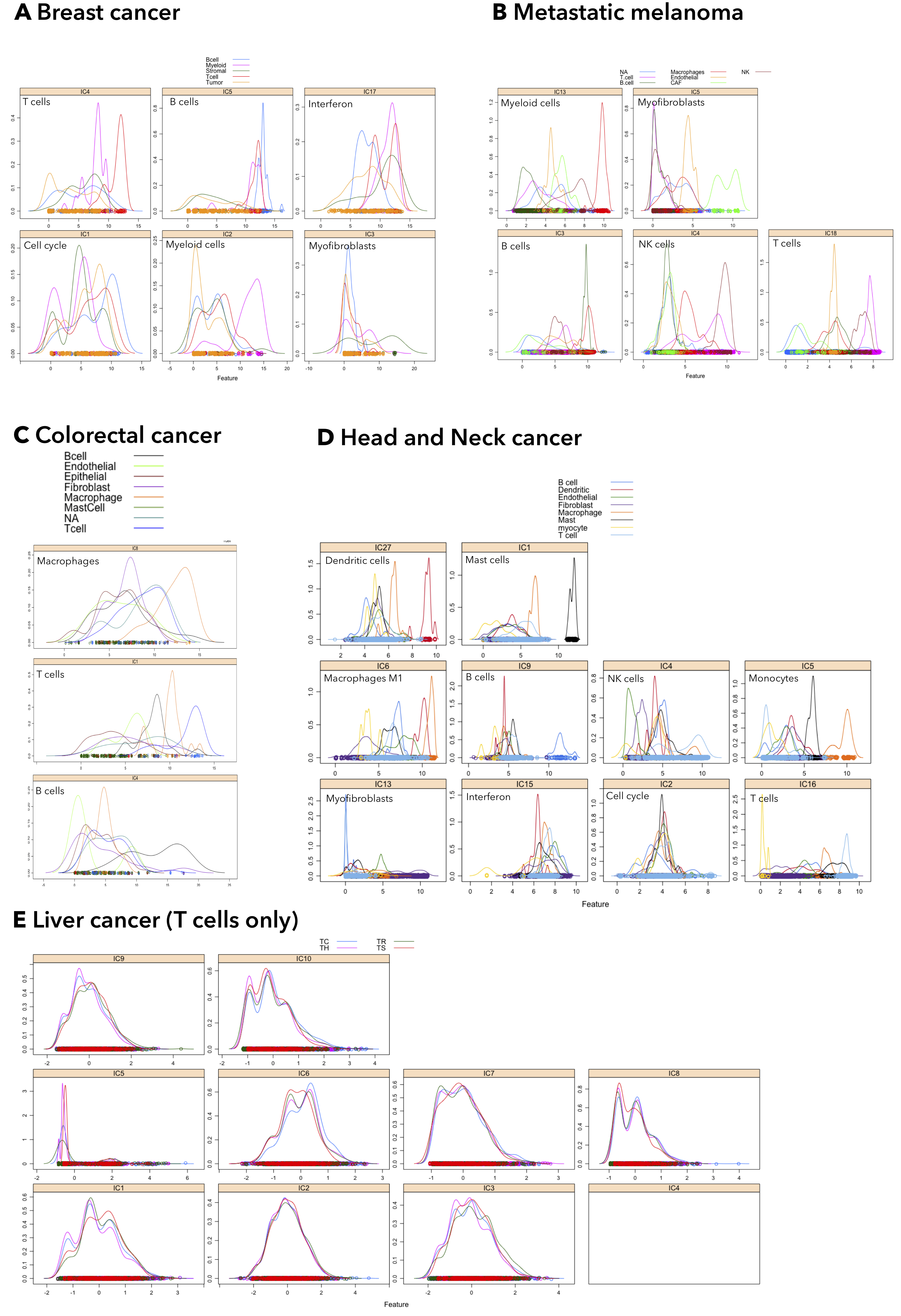
Figure 7.13: ICA applied to scRNA-seq detects cell-specific signatures. Five scRNA-seq datasets (Supplementary table 7.2), were decomposed with ICA into their MSTD (Kairov et al. 2017) dimensions. Cell-type and cellular programs were identified with DeconICA (written label) and confirmed with the author given cell type labels. The density plots show the abundance scores of a selected component distribution over cells. In all datasets except the T cell liver cancer, dataset cell-type components were correctly identified.
7.6.2 Tables
References
Galon, Jérôme, Bernhard Mlecnik, Gabriela Bindea, Helen K Angell, Anne Berger, Christine Lagorce, Alessandro Lugli, et al. 2014. “Towards the introduction of the ‘Immunoscore’ in the classification of malignant tumours.” J. Pathol. 232 (2): 199–209. doi:10.1002/path.4287.
Taube, Janis M, Jérôme Galon, Lynette M Sholl, Scott J Rodig, Tricia R Cottrell, Nicolas A Giraldo, Alexander S Baras, et al. 2017. “Implications of the tumor immune microenvironment for staging and therapeutics.” Mod. Pathol. doi:10.1038/modpathol.2017.156.
Zou, Weiping, Jedd D. Wolchok, and Lieping Chen. 2016. “PD-L1 (B7-H1) and PD-1 pathway blockade for cancer therapy: Mechanisms, response biomarkers, and combinations.” Sci. Transl. Med. 8 (328). doi:10.1126/scitranslmed.aad7118.
Topalian, Suzanne L., Janis M. Taube, Robert A. Anders, and Drew M. Pardoll. 2016. “Mechanism-driven biomarkers to guide immune checkpoint blockade in cancer therapy.” Nat. Rev. Cancer 16 (5). Nature Publishing Group: 275–87. doi:10.1038/nrc.2016.36.
Wong, Michael Thomas, David Eng Hui Ong, Frances Sheau Huei Lim, Karen Wei Weng Teng, Naomi McGovern, Sriram Narayanan, Wen Qi Ho, et al. 2016. “A High-Dimensional Atlas of Human T Cell Diversity Reveals Tissue-Specific Trafficking and Cytokine Signatures.” Immunity 45 (2): 442–56. doi:10.1016/j.immuni.2016.07.007.
De Simone, Marco, Alberto Arrigoni, Grazisa Rossetti, Paola Gruarin, Valeria Ranzani, Claudia Politano, Raoul J.P. Bonnal, et al. 2016. “Transcriptional Landscape of Human Tissue Lymphocytes Unveils Uniqueness of Tumor-Infiltrating T Regulatory Cells.” Immunity 45 (5). Cell Press: 1135–47. doi:10.1016/J.IMMUNI.2016.10.021.
Plitas, George, Catherine Konopacki, Kenmin Wu, Paula D. Bos, Monica Morrow, Ekaterina V. Putintseva, Dmitriy M. Chudakov, and Alexander Y. Rudensky. 2016. “Regulatory T Cells Exhibit Distinct Features in Human Breast Cancer.” Immunity 45 (5). Cell Press: 1122–34. doi:10.1016/J.IMMUNI.2016.10.032.
Chen, Daniel S., and Ira Mellman. 2017. “Elements of cancer immunity and the cancer-immune set point.” doi:10.1038/nature21349.
Becht, Etienne, Aurélien de Reyniès, Nicolas A Giraldo, Camilla Pilati, Bénédicte Buttard, Laetitia Lacroix, Janick Selves, Catherine Sautès-Fridman, Pierre Laurent-Puig, and Wolf Herman Fridman. 2016. “Immune and Stromal Classification of Colorectal Cancer Is Associated with Molecular Subtypes and Relevant for Precision Immunotherapy.” Clin. Cancer Res. 22 (16). American Association for Cancer Research: 4057–66. doi:10.1158/1078-0432.CCR-15-2879.
Newman, Aaron M, Chih Long Liu, Michael R Green, Andrew J Gentles, Weiguo Feng, Yue Xu, Chuong D Hoang, Maximilian Diehn, and Ash A Alizadeh. 2015. “Robust enumeration of cell subsets from tissue expression profiles.” Nat. Methods 12 (5). Nature Publishing Group: 453–57. doi:10.1038/nmeth.3337.
Aran, Dvir, Zicheng Hu, and Atul J. Butte. 2017. “xCell: digitally portraying the tissue cellular heterogeneity landscape.” Genome Biol. 18 (1). BioMed Central: 220. doi:10.1186/s13059-017-1349-1.
Racle, Julien, Kaat de Jonge, Petra Baumgaertner, Daniel E Speiser, and David Gfeller. 2017. “Simultaneous enumeration of cancer and immune cell types from bulk tumor gene expression data.” Elife 6. eLife Sciences Publications Limited: e26476. doi:10.7554/eLife.26476.
Chifman, Julia, Ashok Pullikuth, Jeff W Chou, Davide Bedognetti, and Lance D Miller. 2016. “Conservation of immune gene signatures in solid tumors and prognostic implications.” BMC Cancer 16 (1): 911. doi:10.1186/s12885-016-2948-z.
Cheng, Wei-Yi, Tai-Hsien Ou Yang, and Dimitris Anastassiou. 2013. “Biomolecular Events in Cancer Revealed by Attractor Metagenes.” Edited by Isidore Rigoutsos. PLoS Comput. Biol. 9 (2). Public Library of Science: e1002920. doi:10.1371/journal.pcbi.1002920.
Cieślik, Marcin, and Arul M. Chinnaiyan. 2017. “Cancer transcriptome profiling at the juncture of clinical translation.” Nat. Rev. Genet. 19 (2). Nature Publishing Group: 93–109. doi:10.1038/nrg.2017.96.
Repsilber, Dirk, Sabine Kern, Anna Telaar, Gerhard Walzl, Gillian F Black, Joachim Selbig, Shreemanta K Parida, Stefan HE Kaufmann, and Marc Jacobsen. 2010. “Biomarker discovery in heterogeneous tissue samples -taking the in-silico deconfounding approach.” BMC Bioinformatics 11 (1). BioMed Central: 27. doi:10.1186/1471-2105-11-27.
Gaujoux, Renaud, and Cathal Seoighe. 2012. “Semi-supervised Nonnegative Matrix Factorization for gene expression deconvolution: A case study.” Infect. Genet. Evol. 12 (5). Elsevier: 913–21. doi:10.1016/J.MEEGID.2011.08.014.
Wang, Niya, Eric P. Hoffman, Lulu Chen, Li Chen, Zhen Zhang, Chunyu Liu, Guoqiang Yu, David M. Herrington, Robert Clarke, and Yue Wang. 2016. “Mathematical modelling of transcriptional heterogeneity identifies novel markers and subpopulations in complex tissues.” Sci. Rep. 6 (1). Nature Publishing Group: 18909. doi:10.1038/srep18909.
Czerwinska, Urszula. 2018. “UrszulaCzerwinska/DeconICA: DeconICA first release.” doi:10.5281/ZENODO.1250070.
Biton, Anne, Isabelle Bernard-Pierrot, Yinjun Lou, Clémentine Krucker, Elodie Chapeaublanc, Carlota Rubio-Pérez, Nuria López-Bigas, et al. 2014. “Independent Component Analysis Uncovers the Landscape of the Bladder Tumor Transcriptome and Reveals Insights into Luminal and Basal Subtypes.” Cell Rep. 9 (4): 1235–45. doi:10.1016/j.celrep.2014.10.035.
Cantini, Laura, Ulykbek Kairov, Aurelien de Reynies, Emmanuel Barillot, Francois Radvanyi, and Andrei Zinovyev. 2018. “Stabilized Independent Component Analysis outperforms other methods in finding reproducible signals in tumoral transcriptomes.” bioRxiv. Cold Spring Harbor Laboratory, 318154. doi:10.1101/318154.
Chen, Edward Y, Christopher M Tan, Yan Kou, Qiaonan Duan, Zichen Wang, Gabriela Meirelles, Neil R Clark, and Avi Ma’ayan. 2013. “Enrichr: interactive and collaborative HTML5 gene list enrichment analysis tool.” BMC Bioinformatics 14 (1): 128. doi:10.1186/1471-2105-14-128.
Hänzelmann, Sonja, Robert Castelo, and Justin Guinney. 2013. “GSVA: gene set variation analysis for microarray and RNA-Seq data.” BMC Bioinformatics 14 (1). BioMed Central: 7. doi:10.1186/1471-2105-14-7.
Wagner, Florian, Yun Yan, and Itai Yanai. 2018. “K-nearest neighbor smoothing for high-throughput single-cell RNA-Seq data.” bioRxiv. Cold Spring Harbor Laboratory, 217737. doi:10.1101/217737.
Kairov, Ulykbek, Laura Cantini, Alessandro Greco, Askhat Molkenov, Urszula Czerwinska, Emmanuel Barillot, and Andrei Zinovyev. 2017. “Determining the optimal number of independent components for reproducible transcriptomic data analysis.” BMC Genomics 18 (1). BioMed Central: 712. doi:10.1186/s12864-017-4112-9.
Thorsson, Vésteinn, David L Gibbs, Scott D Brown, Denise Wolf, Dante S Bortone, Tai-Hsien Ou Yang, Eduard Porta-Pardo, et al. 2018. “The Immune Landscape of Cancer.” Immunity 48 (4). Elsevier: 812–830.e14. doi:10.1016/j.immuni.2018.03.023.
Tamborero, David, Carlota Rubio-Perez, Ferran Muinos, Radhakrishnan Sabarinathan, Josep Maria Piulats, Aura Muntasell, Rodrigo Dienstmann, Nuria Lopez-Bigas, and Abel Gonzalez-Perez. 2018. “A pan-cancer landscape of interactions between solid tumors and infiltrating immune cell populations.” Clin. Cancer Res. American Association for Cancer Research, clincanres.3509.2017. doi:10.1158/1078-0432.CCR-17-3509.
Newberg, Lee A., Xiaowei Chen, Chinnappa D. Kodira, and Maria I. Zavodszky. 2018. “Computational de novo discovery of distinguishing genes for biological processes and cell types in complex tissues.” Edited by Paolo Provero. PLoS One 13 (3). Public Library of Science: e0193067. doi:10.1371/journal.pone.0193067.
Ogundijo, Oyetunji E., and Xiaodong Wang. 2017. “A sequential Monte Carlo approach to gene expression deconvolution.” Edited by Lars Kaderali. PLoS One 12 (10). Public Library of Science: e0186167. doi:10.1371/journal.pone.0186167.
Moffitt, Richard A, Raoud Marayati, Elizabeth L Flate, Keith E Volmar, S Gabriela Herrera Loeza, Katherine A Hoadley, Naim U Rashid, et al. 2015. “Virtual microdissection identifies distinct tumor- and stroma-specific subtypes of pancreatic ductal adenocarcinoma.” Nat. Genet. 47 (10). Nature Publishing Group: 1168–78. doi:10.1038/ng.3398.
Brunet, Jean-Philippe, Pablo Tamayo, Todd R Golub, and Jill P Mesirov. 2004. “Metagenes and molecular pattern discovery using matrix factorization.” Proc. Natl. Acad. Sci. U. S. A. 101 (12). National Academy of Sciences: 4164–9. doi:10.1073/pnas.0308531101.
Paulson, Joseph N, Cho-Yi Chen, Camila M Lopes-Ramos, Marieke L Kuijjer, John Platig, Abhijeet R Sonawane, Maud Fagny, Kimberly Glass, and John Quackenbush. 2017. “Tissue-aware RNA-Seq processing and normalization for heterogeneous and sparse data.” BMC Bioinformatics 18 (1). BioMed Central: 437. doi:10.1186/s12859-017-1847-x.
Zheng, Chunhong, Liangtao Zheng, Jae-Kwang Yoo, Huahu Guo, Yuanyuan Zhang, Xinyi Guo, Boxi Kang, et al. 2017. “Landscape of Infiltrating T Cells in Liver Cancer Revealed by Single-Cell Sequencing.” Cell 169 (7). Cell Press: 1342–1356.e16. doi:10.1016/J.CELL.2017.05.035.
Schelker, Max, Sonia Feau, Jinyan Du, Nav Ranu, Edda Klipp, Birgit Schoeberl, Gavin MacBeath, et al. 2017. “Estimation of immune cell content in tumour tissue using single-cell RNA-seq data.” Nat. Commun. 8 (1). Nature Publishing Group: 2032. doi:10.1038/s41467-017-02289-3.
Tirosh, Itay, Benjamin Izar, Sanjay M. Prakadan, Marc H. Wadsworth, Daniel Treacy, John J. Trombetta, Asaf Rotem, et al. 2016. “Dissecting the multicellular ecosystem of metastatic melanoma by single-cell RNA-seq.” Science (80-. ). 352 (6282): 189–96. doi:10.1126/science.aad0501.
Cantini, Laura, Laurence Calzone, Loredana Martignetti, Mattias Rydenfelt, Nils Blüthgen, Emmanuel Barillot, and Andrei Zinovyev. 2018. “Classification of gene signatures for their information value and functional redundancy.” Npj Syst. Biol. Appl. 4 (1). Nature Publishing Group: 2. doi:10.1038/s41540-017-0038-8.
Görtler, Franziska, Stefan Solbrig, Tilo Wettig, Peter J. Oefner, Rainer Spang, and Michael Altenbuchinger. 2018. “Loss-function learning for digital tissue deconvolution.” http://arxiv.org/abs/1801.08447.
Kharchenko, Peter V, Lev Silberstein, and David T Scadden. 2014. “Bayesian approach to single-cell differential expression analysis.” Nat. Methods 11 (7). Nature Publishing Group: 740–42. doi:10.1038/nmeth.2967.
Svensson, Valentine, Roser Vento-Tormo, and Sarah A Teichmann. 2018. “Exponential scaling of single-cell RNA-seq in the past decade.” Nat. Protoc. 13 (4). Nature Publishing Group: 599–604. doi:10.1038/nprot.2017.149.
Weinstein, John N, Eric A Collisson, Gordon B Mills, Kenna R Mills Shaw, Brad A Ozenberger, Kyle Ellrott, Ilya Shmulevich, et al. 2013. “The Cancer Genome Atlas Pan-Cancer Analysis Project.” Nature Genetics 45 (10). Nature Publishing Group: 1113.
Edgar, Ron, Michael Domrachev, and Alex E Lash. 2002. “Gene Expression Omnibus: NCBI gene expression and hybridization array data repository.” Nucleic Acids Res. 30 (1): 207–10. http://www.ncbi.nlm.nih.gov/pubmed/11752295 http://www.pubmedcentral.nih.gov/articlerender.fcgi?artid=PMC99122.
Kolesnikov, Nikolay, Emma Hastings, Maria Keays, Olga Melnichuk, Y Amy Tang, Eleanor Williams, Miroslaw Dylag, et al. 2015. “ArrayExpress update–simplifying data submissions.” Nucleic Acids Res. 43 (Database issue): D1113–6. doi:10.1093/nar/gku1057.
Chung, Woosung, Hye Hyeon Eum, Hae-Ock Lee, Kyung-Min Lee, Han-Byoel Lee, Kyu-Tae Kim, Han Suk Ryu, et al. 2017. “Single-cell RNA-seq enables comprehensive tumour and immune cell profiling in primary breast cancer.” Nat. Commun. 8. Nature Publishing Group: 15081. doi:10.1038/ncomms15081.
Baker, Monya. 2012. “Quantitative data: learning to share.” Nat. Methods 9 (1): 39–41. doi:10.1038/nmeth.1815.
Durinck, Steffen, Paul T Spellman, Ewan Birney, and Wolfgang Huber. 2009. “Mapping identifiers for the integration of genomic datasets with the R/Bioconductor package biomaRt.” Nat. Protoc. 4 (8): 1184–91. doi:10.1038/nprot.2009.97.
Shannon, P., Andrew Markiel, Owen Ozier, Nitin S Baliga, Jonathan T Wang, Daniel Ramage, Nada Amin, Benno Schwikowski, and Trey Ideker. 2003. “Cytoscape: A Software Environment for Integrated Models of Biomolecular Interaction Networks.” Genome Res. 13 (11): 2498–2504. doi:10.1101/gr.1239303.
Stacklies, W., H. Redestig, M. Scholz, D. Walther, and J. Selbig. 2007. “pcaMethods a bioconductor package providing PCA methods for incomplete data.” Bioinformatics 23 (9). Oxford University Press: 1164–7. doi:10.1093/bioinformatics/btm069.
Porta, J.M., J.J. Verbeek, and B.J.A. Kröse. 2005. “Active Appearance-Based Robot Localization Using Stereo Vision.” Auton. Robots 18 (1): 59–80. doi:10.1023/B:AURO.0000047287.00119.b6.
Cai, Jian-Feng, Emmanuel J Candès, and Zuowei Shen. 2008. “A Singular Value Thresholding Algorithm for Matrix Completion.” https://arxiv.org/pdf/0810.3286v1.pdf.
Troyanskaya, Olga, Michael Cantor, Gavin Sherlock, Pat Brown, Trevor Hastie, Robert Tibshirani, David Botstein, and Russ B Altman. 2001. “Missing value estimation methods for DNA microarrays.” BIOINFORMATICS 17 (6): 520–25. https://academic.oup.com/bioinformatics/article-abstract/17/6/520/272365.
Van Der Maaten, Laurens, and Geoffrey Hinton. 2008. “Visualizing Data using t-SNE.” J. Mach. Learn. Res. 9: 2579–2605. https://lvdmaaten.github.io/publications/papers/JMLR{\_}2008.pdf.
Mcinnes, Leland, and John Healy. 2018. “UMAP: Uniform Manifold Approximation and Projection for Dimension Reduction.” https://arxiv.org/pdf/1802.03426.pdf.
Becht, Etienne, Charles-Antoine Dutertre, Immanuel W.H. Kwok, Lai Guan Ng, Florent Ginhoux, and Evan W Newell. 2018. “Evaluation of UMAP as an alternative to t-SNE for single-cell data.” bioRxiv. Cold Spring Harbor Laboratory, 298430. doi:10.1101/298430.
Hopkins, Brian. 1954. “A New Method for determining the Type of Distribution of Plant Individuals.” Ann. Bot. 18 (70): 213–26. doi:10.1093/aob/.
Wickham, Hadley. 2016. Ggplot2: Elegant Graphics for Data Analysis. Springer-Verlag New York. http://ggplot2.org.
Kolde, Raivo. 2018. Pheatmap: Pretty Heatmaps. https://CRAN.R-project.org/package=pheatmap.
Auguie, Baptiste. 2017. GridExtra: Miscellaneous Functions for “Grid” Graphics. https://CRAN.R-project.org/package=gridExtra.
Sarkar, Deepayan. 2008. Lattice: Multivariate Data Visualization with R. New York: Springer. http://lmdvr.r-forge.r-project.org.
Sievert, Carson, Chris Parmer, Toby Hocking, Scott Chamberlain, Karthik Ram, Marianne Corvellec, and Pedro Despouy. 2017. Plotly: Create Interactive Web Graphics via ’Plotly.js’. https://CRAN.R-project.org/package=plotly.